Lifetime Value Prediction: A Mode vs Mean problem

Even the greatest can be wrong. In this project I tell part of my experience with an incredible Google paper, and how I improved it by correcting a simple fundamental mistake. This post shows how important it is to always go back to basics and think simple.

Project in prediction of LTV (Lifetime Value) of the individual clients. Based on the behavior of users in the application, predict if they are going to return, if they are going to make a payment and estimate the amount. The problem is especially complex due to the skewed distribution, where the majority of users are non-payers.

I start working in this project at February of 2022 and extended for four months. It is one of the most challenging problems I faced in the recent years. The final objective is to predict the quality of new users by predicting how much they are going to spend, based on the actions that this user has taken in the past. Having little time frame to take action on campaigns. In this post I will expose some of the challenges and my personal experience with this hard LTV prediction problem.

Main Challenges

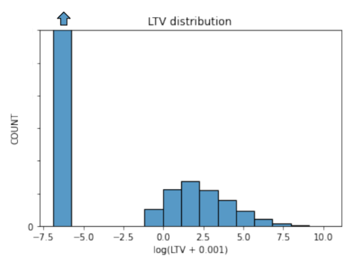
Very large proportion of users are non-payers, so the LTV distribution is heavily tailed (see next figure).
Short amount of time to understand new users behavior in order to take action.

Figure: The LTV distribution is very heavily tailed. The big bar on the left represent non-payers, and the rest correspond to the distribution for the payers.

Research

When I’m facing a new challenging problem, the first step that I always take is to look into the literature. The first and most remarkable result that I found was the paper “A Deep Probabilistic Model for Customer Lifetime Value Prediction”. At first, as for every paper, it was hard to understand everything till I find a post of Maja Pavlovic explaining the idea more easily.

The highly imbalance between payers and non-payers users is very hard for a regression problem, if it where only a classification problem it can be managed using weighted loss function or any of the others well know methods. But at the end, the final objective of the LTV prediction is a regression problem of determine the total amount that a user will spend, and not the simpler classification problem alone. But given the extreme imbalance in the data, the classical approach didn’t allow to predict correctly how much a user was going to spend.

Basically the Gauss distribution hypothesis for the output variable is not adequate for this problem, which is directly related to L1 or L2 loss functions. Also, in trying to generalize better and prevent overfit, ML models tends to smooth over the outliers (the paying users). In other words, the extreme imbalance in the data with only a small fraction of payers, produce that the model tends to output a value of zero for every prediction. This leads to a very small average error because almost all clients where non-payers, and even paying clients didn’t spend big amounts of money (so the trend of the model is to zero).

On the other hand, In this initial research I also learned that the more common approach for LTV prediction is to train two models, one for classification and other for the regression of the payers. I tried many models, but finally the best was XGBoost for both models. Also, I discover that the best way of doing this is to put the two models in tandem, one before the other. First the classifier, and then the regressor only trained for paying users. But I still wanted to try the paper approach and see if it can work better (or simply have a reference for comparison). Have to say that in Structured ML problems is general very complicated to determine a benchmark, as compared to unstructured problems in which humans are the common ground truth.

Short explanation of the paper

I simply love the paper and wanted to try it, for the time it was very recent and it promise a lot. The idea of the paper was to leave the Gaussian assumption of the target variable (which wasn’t true anyway) and define a more adequate loss function. The idea was to combine the classification and the regression models into a single unique model, given raise to a more complex loss function that represents the highly imbalance distribution. See the next figure.

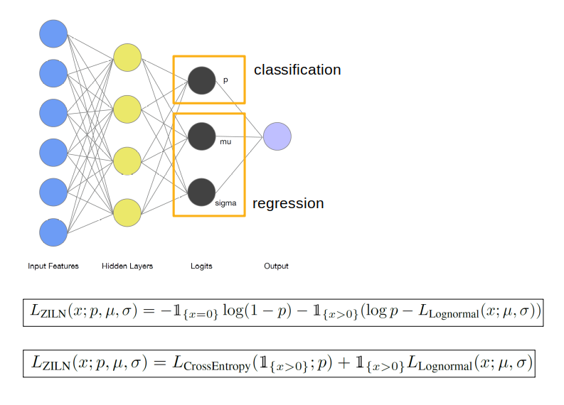
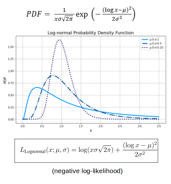
Figure: The Neural Network which in the final layer outputs the parameters of the distribution for both models. Notice that the loss function is a combination of both the classification and the regression model. Figure adapted from the original paper.

Note that regression part of the model needs the output the parameter sigma which is necessary for the prediction of the Log-normal distribution, which is the correct distribution for paying users (this parameter is not needed in the classic Gaussian distribution prediction). To see this in a more mathematical way, and determine the loss function associated for a Log-normal distribution, the key is on the maximum likelihood estimation. See the next figure.

Figure: The likelihood is the multiplication of all the P(X_i | mu, sigma) for every sample. But it is simply more easy to add than multiply, so is common to take the logarithm of the likelihood. The logarithm preserves the same objective function because it is a monotonic function. Also, they add a minus sign to minimize instead of maximize the likelihood. All this give raise to the negative log likelihood for the distribution for the payers (which is supposed to be a log normal distribution). Figure adapted from Maja Pavlovic blog article.

Facing the real problem

So the idea and the theory is amazing, but it has some practical problems.

The model use in the paper is a very deep Neural Network, which based in my experience was too big for this problem. It is difficult to calibrate and also leads to overfitting problems. DNN is not in general the first option for structured data problems, despite of being the state of the art in unstructured data problems. This is mainly because they don’t naturally tend look at each variable independently, needs a lot of data, are difficult to calibrate, and in general they don’t work better than other models (specially ensemble tree methods which tends to generalize better with less overfitting). Of course, in same cases DNN can achieve the same or even better results in structured data with the right calibration, but it is not easy and the general rule is that DNN is more the state of the art in unstructured data. But TensorFlow has the amazing practical advantage of being much more flexible than Scikit-learn or XGBoost libraries. In TensorFlow the authors could modify the loss function easily, and probably that was the main reason they used a DNN, but in theory the approach presented in the paper can be used in other type of models and probably DNN isn’t the best option in general (even with the great modify of the loss function).
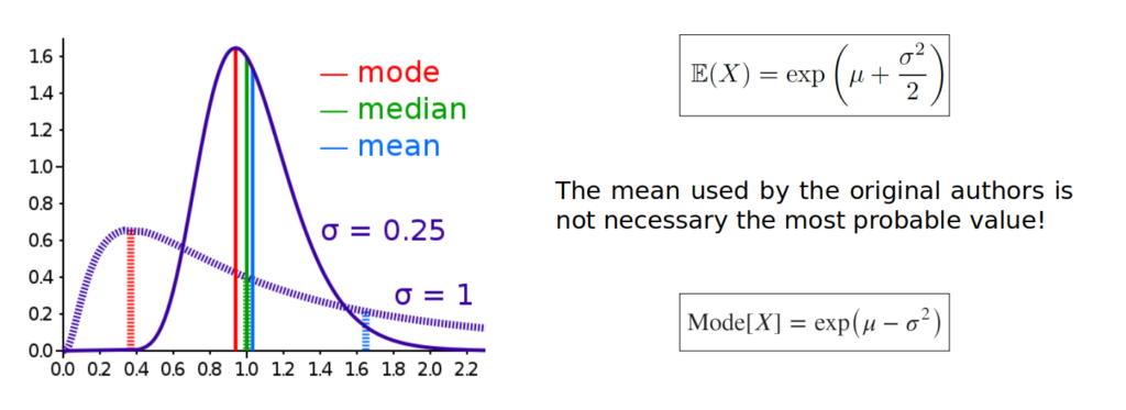
The most important correction, and probably the reason why a write this document, is that for the prediction the authors where using the mean value. But the mean is not necessarily the most probable value, which is really the mode (the value X that makes a maximum in the distribution). The confusion raises because in the common Gaussian distribution they are the same (being a symmetric distribution) so it doesn’t make any a difference. Also the mean is misleadingly know as expected value which adds to this common confusion. In the project that I was working, find a great improvement in the model by the correction of this prediction formula in the code. See the next figure.

Figure: The mean for a log-normal distribution is not the mode, the most probable value. Actually they can be very different, altering the predictions. This doesn’t make a difference in the training stage, only in the prediction and the final metrics. Figure adapted from Wikipedia.

Discussion

So the idea behind this paper is great, I simply loved as a method, but it still has a lot of room for improvement. Some future ideas could be making a hyper-parameter lambda that controls the contribution weight between the classification and regression loss (as used in cGAN) or use a sample weight function to given more weight to the payers (the less common class) in the loss function, taken more advantage of the classification part of the model. Because now it seems that the only objective of the paper was to combine two model into one for operational purposes, but not for the objective of improving metrics.

But for now, I corrected the Mode vs Mean in the TensorFlow code with amazing results, it actually works much better than the original code. Is amazing how a simple statistical concept could lead very rapidly to much better results.

Tools: Python, Git, SQL, Pandas, TensorFlow, Keras, CUDA/GPU, XGBoost, Scikit-Learn, Matplotlib, Seaborn.