The most common mistake in Machine Learning: How to quantify uncertainty? Likelihood vs Confidence

About

I started writing this post because of the most common misconception that I have always found in Machine Learning, almost always causing some practical problems. But the truth is that I extended the post much more and ended up becoming also one about how to measure the uncertainty of a prediction. This is not just having the general metrics of the model, but knowing how confident you are about a particular prediction. Some situations can be more difficult to predict than others, and it is very useful to be able to know the level of confidence. It is a very important issue to know when we can trust a model, in any industry it can be critical. The subject has taken great importance in the last time but it is not treated correctly by many traditional courses. Being of particular importance in unstructured data problems, where the randomness of the data is greater in general. I must say that even certain modern ML libraries like Scikit-learn do not provide adequate functionality for this purpose.

Introduction

In every single company that I worked, I have found the same problem over and over again, which motivates this small post. The first time that I encountered this problem was while working on Medical Imaging for one of the biggest hospitals in the country. The concrete project was an image classification detector for a certain disease. So at the end of the project, the problems started when deciding what was the best way of presenting the results of the predictions to the medical professionals. The thing is that certain models, as logistic regression and neural networks, can output a certain probability for each class. But in the wrong interpretation of this probability is when the real misconceptions started.

The practical problem presented in the hospital was that, even though we claim to have a 0.92 for model accuracy, for a particular input sample the output model probability was 0.65 which is very difficult to interpret for a health worker which is not an expert on Machine Learning. We received very soon questions of whether 0.65 means that the person has or has not covid and what should they do with this information. Is this 0.65 means that it has a little covid, being only little over 0.5? Maybe it is in an early stage of the disease?. Or it is that this 0.65 means that the person has 65 % of the lung with covid?. After all this questions my boss decided that I was right and we only should output the final prediction as every medical test result, only based on a binary positive or negative result.

Knowing the confidence of a prediction is of particular importance in medical applications, but it is not a rare exception, and in almost every industry is something of grate value. In the recent years has taken a lot of importance and many research is done in the subject. In this post I will explain the origin of this misconception, how this model probability is really useful, and how to really quantify model uncertainty.

The Origin of Model Probabilities

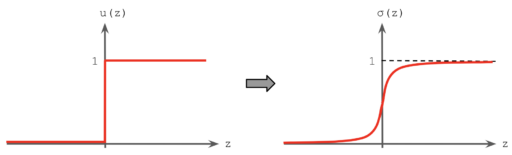
The story behind the origin of this probabilities in classification tasks for certain models, in particular Neural Networks, is that at the end the predictions are a categorical discrete problem. But backpropagation / gradient decent algorithm used to train the model weights, depends on derivatives and the chain rule. So the numerical optimization requires a not-null derivate for the function as an output to make the computations. For this purpose some activation functions where invented, sigmoid and softmax. Both of this activation functions outputs numbers between zero and one, emulating the categorial probability distribution of the output. Also, both of them has exponential functions in their formulas, which is the only function which its derivative is itself (making it easy to take the derivatives) and also can represent the rapid and abrupt changes between the zero and one values (exponentials grows very fast) in trying to emulate the discrete nature of the real output. See figure 1.

Figure 1: The sigmoid activation function σ(z) = 1 / (1 + exp(-z)) is a continue derivable approximation of a discrete step function, which is the real binary domain of the output.

The general problems

This activations functions are mathematically convenient, but are not written in stone and are model dependent (actually many models don’t output any probability). But it is true that this model probability, the sigmoid function, represent a distance to the decision boundary frontier of the model for a particular sample. For example, if the output value is 0.5 the sample is on the boundary. If we have two samples, one with output model probability of 0.7 and the other of 0.9, it means that the first one is more closed to the decision boundary of the model. Part of the misleading in the confidence interpretation is in this non linear relation between the distance to the decision boundary and the model probability. They argue that the confidence in the prediction increases if they are further away from the decision boundary of the model. Even though it could be consider as an indicator, the truth is that it is not necessarily true and has many problems. See figure 2.

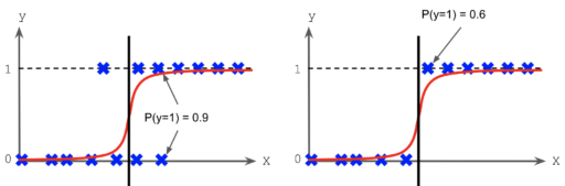
Figure 2: On the right the two categories are perfectly separable, so even an output probability of 0.6 is enough for be certain about the output. On the left the two categories are not perfectly separable, so even a probability of 0.9 is not enough to be certain. This is due to uncertainty in the data which can not be improved by getting more training data, only by new features may this situation improve (which is not always possible in practice).

The level of uncertainty is not same across the decision boundary (also the frontier is in general different for every model).
Even with a model probability of 0.6 could be enough to be completely certain of the output, supposing that the metrics of the model are sufficiently good. If the two sets are separable, and the model is well trained, even a 0.6 is enough for getting a correct detection.
If the data uncertainty is sufficiently high, even an output probability of 0.9 is not sufficient for being certain about the output. Have to say that is very common that the classification sets are not perfectly separable by the input variables.
Is very hard for a model to quantify its own uncertainty for a particular input, because the problem is in itself. If the quality of the model is no sufficient, it can’t be trusted the output model probability.

For a more practical example of this misconception, consider the typical case of having to classify between two mutually exclusive categories, could be Cat vs Dog classifier. Suppose that both of this categories are present in the input image, then a well trained model will give a probability very nearly to 0.5, which in the probability interpretation means that the model is very unsure about the output, but in reality it is actually very confident. See figure 3.

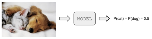
Figure 3: The output probability of a perfect classification model is 0.5 if the two classes are present in the input.

Have to say that this example is just for illustration purposes, the mutually exclusive hypothesis could very easily relax by changing the output layer structure and activation function (or even training a separate model for each category). For example, for a two units output layer, softmax enforces that all probabilities outputs for each category adds to one, by simply changing it to a sigmoid the output probabilities doesn’t necessarily have to add to one in the final layer.

But the previous problem doesn’t stop there, and there are more complex scenarios. For example, if now we pass the model an image of a Car, which is not one of the original classes, the output probability could be very easily an extreme value, for example 0.9. Which could lead to think that the model is very confident about the output (but clearly a Car is not a Dog or a Cat). See figure 4. This extreme value in the probability is mainly because the image is very different from the training distribution and could be very far from the model decision boundary.

Figure 4: The model appears to be very certain about the image is a Dog but it is not the case.

Of curse this are not problems exclusively for images, which is used in this post simply for illustration purposes. Other simple possible example would be a classifier between English and Spanish for detecting the language present in a text, if both are partially present in the input text, the output would be 0.5 but the confidence that both are present could be very high. Also, if you have an unknown language for the model, it can also output a misleading very high or low probability.

Then, what is the use of this model probability?

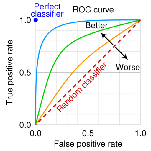
There is one very important application of this model probability, which is in the trade off between the true and false positive rates for a trained model. By default the threshold for a classification model is 0.5, but for a particular application, depending on the needs of the company, this threshold can be set higher or lower. With the adjustment of this threshold the precision vs recall proportion can be changed, informally “the amount vs quality of the detections”.

In practice, playing with this threshold value to improve a metric can affect negatively all other metrics. The ROC curve plot is construct for tune more easily this threshold, so graphically select the best option for the company use case. Also the ROC curve can be use to know how robust is the model to changes in this threshold by calculating the area under the curve (AUC), which is a number between 0.5 and 1. See figure 5.

Figure 5: The ROC curve shows the True Positive vs False Positive rate for different values of the threshold. The are under the ROC curve AUC is 0.5 for a random classifier and 1 for a perfect classifier. Image taken from Wikipedia.

How to really quantify uncertainty

This could easily be another post, in the sense that has much more mathematical details. But due to the recent interest to know the uncertainty of the models, which is not provided by many libraries as Scikit-learn, is that I included it in this post. Maybe in the future is going to became very common, but today is not very clear for many professionals and is a very important topic. You need to know how certain is a prediction to take better actions.

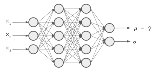
One of the faster and simpler ways of quantifying data uncertainty for a particular input (and not just have the general metrics of the model), is to make the model directly estimate the variance from the input and not only the expected value for the prediction. For this, we are going to modify the typical loss function by using the maximum likelihood estimation method for a regression problem. Just for make the discussion more concrete we are going to use a Neural Net (but this method is not exclusive to Neural Nets). See Figure 6.

Figure 6: A Neural Network that outputs both the expected value prediction and the uncertainty.

The least square is the common approach for training ML models, by simply minimizing the sum of squares of the errores (the square of the differences between the predictions and the real value). This is related to maximum likelihood estimation method by the Gaussian distribution with constant variance assumption of the individual independent samples. Actually, under this conditions, the maximum likelihood estimation gives exactly the traditional loss.

The Likelihood represent the joint probability density function of $(y_1, y_2, \ldots , y_N)$ . The independence assumption is key for separating this into a series of multiplication of the individual Gaussian distributions for each sample. The objective (or the idea) is to maximize this joint probability of every sample given the Gaussian distribution shape assumption (define completely by the parameters $\mu$ and $\sigma$ ). Let me show you in more detail, here is the maximum likelihood estimation method for a set of $N$ training samples:

$\max \prod_{i=1}^N f(y_i |\mu_i , \sigma)$

where

$f(y_i |\mu , \sigma)=\frac{1}{\sqrt{2\pi} \sigma} \exp\left(-\frac{(y_i-\mu_i)^2}{2\sigma^2}\right)$

Knowing that $\mu_i=\hat{y}_i$ is the classical prediction output of the model ( $\text{MODEL}(X_i)=\hat{y}_i$ ). This is because the mode is equal to the mean in a normal distribution (its maximum value is in the mean, this due to the symmetrical shape of the distribution), so the expected value $\mu$ is the prediction $\hat{y}$ . See figure 7.

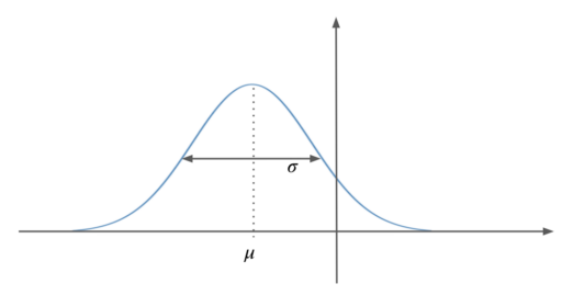Figure 7: A typical Gaussian distribution. Note that uncertainty is model by $\sigma$ and that the mode (which is the most probable value, where the maximum of the distribution is reached) is the same as the mean value due to the symmetrical shape of the distribution.

For maximizing this probability (likelihood), under the assumption of constant $\sigma$ , the result is equivalent to minimize $\sum_{i=1}^N (y_i-\hat y_i)^2$ . This is mainly because of the property $e^a \cdot e^b = e^{a+b}$ . Let’s see in more detail,

$\max \prod_{i=1}^N f(y_i |\mu_i , \sigma)$

$= \max \prod_{i=1}^N \frac{1}{\sqrt{2\pi} \sigma} \exp\left(-\frac{(y_i-\hat y_i)^2}{2\sigma^2}\right)$

$= \max \frac{1}{(\sqrt{2\pi} \sigma)^N}\prod_{i=1}^N \exp\left(-\frac{(y_i-\hat y_i)^2}{2\sigma^2}\right)$

$= \max \frac{1}{(\sqrt{2\pi} \sigma)^N}\exp\left( \sum_{i=1}^N-\frac{(y_i-\hat y_i)^2}{2\sigma^2}\right)$

$= \max \frac{1}{(\sqrt{2\pi} \sigma)^N}\exp\left( -\frac{1}{2\sigma^2}\sum_{i=1}^N (y_i-\hat y_i)^2\right)$

$=\max - \sum_{i=1}^N (y_i-\hat y_i)^2=\min \sum_{i=1}^N (y_i-\hat y_i)^2$

Now, for quantify data uncertainty just need to also estimate $\sigma$ . So doing the same process as before, but now $\sigma$ is estimated in the output by the model. Instead of maximize the likelihood directly, si more common to minimize the negative log-likelihood. The logarithm is a strictly increasing function for converting the multiplications into additions (which is more efficient for the computations), and for converting the maximization to a minimization just take the negative sign. So the new final loss function is negative log-likelihood. Let’s see in more detail, supposing that the model outputs $\mu_i=\hat y_i$ and $\sigma_i$ .

$\max \prod_{i=1}^N f(y_i |\mu_i , \sigma_i)$

$= \max \prod_{i=1}^N \frac{1}{\sqrt{2\pi} \sigma_i} \exp\left(-\frac{(y_i-\hat y_i)^2}{2\sigma_i^2}\right)$

$= \max\left[\log \prod_{i=1}^N \frac{1}{\sqrt{2\pi} \sigma_i} \exp\left(-\frac{(y_i-\hat y_i)^2}{2\sigma_i^2}\right)\right]$

$= \max\sum_{i=1}^N \log\left(\frac{1}{\sqrt{2\pi} \sigma_i} \exp\left(-\frac{(y_i-\hat y_i)^2}{2\sigma_i^2}\right)\right)$

$= \max\sum_{i=1}^N \log\left(\frac{1}{\sqrt{2\pi} \sigma_i}\right) + \log\left(\exp\left(-\frac{(y_i-\hat y_i)^2}{2\sigma_i^2}\right)\right)$

$= \max\sum_{i=1}^N \left[\log\left(\frac{1}{\sqrt{2\pi} \sigma_i}\right) -\frac{(y_i-\hat y_i)^2}{2\sigma_i^2} \right]$

$= \min \sum_{i=1}^N \left[ \frac{1}{2}\log (2\pi {\sigma_i}^2 ) +\frac{(y_i-\hat y_i)^2}{2\sigma_i^2} \right]$

So with this new loss function, the model can now output $\sigma$ the uncertainty in the data for every new sample. See figure 8. A final technical point is that $\mu \in \mathbb{R}$ , so it doesn’t need an activation function $\mu=z$ . But $\sigma > 0$ (strictly positive) can be model better with an activation function that enforce strictly positive values greater than zero and that it is easy to derivate, so an exponential activation function is a great choice $\sigma=\exp(z)$ (or even a simple ReLu $\sigma=\max(0, z)$ can be used, but doesn’t strictly enforce that the value is greater than zero).

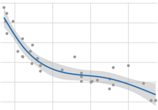Figure 8: Here you can see the data points, with the model predictions in blue, and a confidence interval around it constructed from the Gaussian distribution with the estimated $\sigma$ value. Data source: Motor Trend, 1974.

Have to say that data uncertainty is not the whole history, but model uncertainty is too much for this small post, and for now just suppose the model is good enough and they only uncertainty comes from the data itself. Actually, the approach presented in here is completely valid provided that the model has a large amount of data and is well calibrated.

READ IN MEDIUM