Conditional Generative Adversarial Neural Networks for Metal Artifact Reduction in Spine CT Images

Machine learning is changing the world. One of the most impressive advances are generative models. Over time it will be increasingly difficult to differentiate a fake video, image or audio from a real one. Having fun applications, others very useful, and could even become dangerous due to the generation of fake news content. But one of the most incredible and rare applications is in medical imaging. I had this idea for a post many years ago, but only recently dared to publish it. It is a method for the removal of metallic artifacts in CT images. I wrote it thinking that anyone could read it and find it interesting to some extent, but I must warn that it contains quite a bit of math.

Abstract

Metal objects in Computed Tomography images can produce very severe artifacts that difficult diagnostic and surgical planning. The origin of this artifacts in CT images is due to X-Ray being highly attenuated by metal implants in patients. The objective of this document is presenting a method for attenuating metal artifacts in CT images using a modern approach based on Machine Learning and 3D modeling. Classically, a very common method is to interpolate for reconstructing the missing data of the metal traces, in each 2D slices of the volume of the acquisition space. But only very recently, the use of modern Machine Learning models for completing this acquisition space has come to the attention,[1] instead of the classical non adaptive approaches.

The innovative feature presented in this work is the method in which the training data is created. First get a realistic 3D modeling of the spine directly from CT volume. Second generate and position the metal implants in the 3D model of the spine as a surgeon will do it, instead of the current random approach. Then simulating directly the artifacts produced by replacing the metal lost in the respective acquisition space. This work also wants to present a detailed mathematical theory for new researchers working in the field.

The Data Acquisition Space

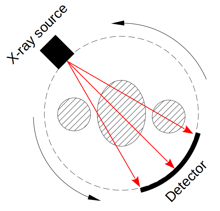
Typical CT scanners works with X-rays, the patient laid in a table slowly enters into a tube, that will capture each slice that will form the final volume. Inside the tube, there is a rotating X-ray source with a detector assembly on the exact opposite side. This X-rays can penetrate through tissues with different levels of absorptions and will generate projections of the body (see figure 1). Then using a mathematical algorithm, from this projections, a digital volume image of the inside of the body emerges.

Figure 1: Schematic representation of the basic operation of a CT scanner. The X-ray source rotates with the detector capturing the projections at every angle while the body enters the machine.

The Radon Transform

Even though there is some differences in the way CT scanners can collect the raw data for the projections, they all can be mapped or modeled to a Radon Transform. For example, single source CT can have different shapes for a detector array (circular arc or collinear) but all can be converted by a simple coordinate transform into parallel beams need for the Radon Transform, also typical multi-slice helical CT can be mapped into a circular CT by interpolation.

So to think, model and program simulations of any typical commercial CT scanner we are going to rely on the Radon Transform and the Filtered Back Projection algorithm to recover the image (the inverse Radon Transform).

For a body with attenuation coefficient $\mu(x,y)$ , the Radon Transform $p_{\theta}(r)$ correspond to the parallel beam projection at an angle $\theta$ (see figure 2). This es given by the equation (1).

(1) $\begin{equation*} p_{\theta}(r) = \int_{-\infty}^{\infty} \mu(x,y) ds = \int_{-\infty}^{\infty} \mu\left(A_{\theta} \begin{bmatrix} r \\ s \end{bmatrix} \right) ds \end{equation*}$

where $\mu(x,y)$ is zero outside the circle of the CT and $A_{\theta}$ is the rotation matrix given by

$A_{\theta}=\begin{bmatrix} \cos\theta & -\sin\theta \\ \sin\theta & \cos\theta \end{bmatrix}.$

Figure 2: Radon Transform $p_{\theta}(r)$ are the projections of parallel beams through an object at every given angel $\theta$ .

The Metal Problem

The relation between the Radon Transform and the real physical intensity capture by the detector is given by Beer-Lambert law, see equation (2).

(2) $\begin{equation*} I_{\theta}(r) = I_0 e^{-p_{\theta}(r)} \end{equation*}$

where $I_0$ is the source intensity. With this, we can rearrange the equation (2) and get the following relation in a more suggestive way for modeling metal, see equation (3).

(3) $\begin{equation*} p_{\theta}(r) = \ln\left(\frac{I_0}{I_{\theta}(r)}\right) = \int_{-R}^{R} \mu(x,y)dz \end{equation*}$

With this relation is more easy to see the behaviour of metal and problem with the reconstruction algorithm. For both air and metal, from equation (3) it can be deduced that:

Air:
$I_{\theta}(r) = I_0 \ \Rightarrow \ p_{\theta}(r) = 0 \ \Rightarrow \ \mu(x,y) = 0$
Metal:
$I_{\theta}(r) = 0 \ \Rightarrow \ p_{\theta}(r) \to +\infty \ \Rightarrow \ \mu(x,y) \to +\infty$
at least for some region of $(x,y)$ .

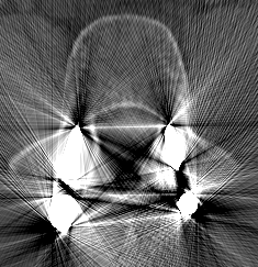
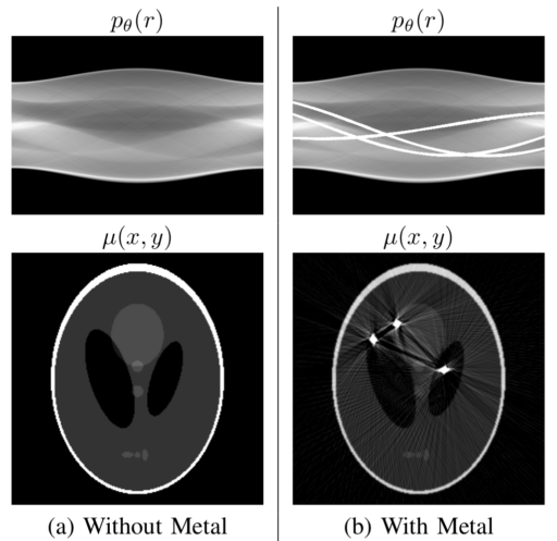
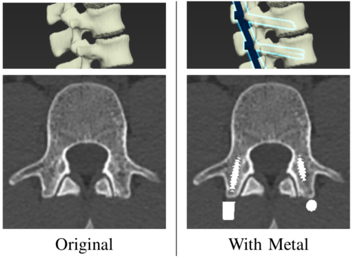
This infinite value for metal is the problem both for the computer representation and the theory. The problem arises because all the information that is in the line of beam that passes trough the metal is lost. Every object in the beam line of a metal is hidden from the detector and produces artifacts in the reconstruction (see figure 3).

Also, notice that to know where the metal traces are going to be, is just a matter of segmenting the metal traces with a simple threshold do to the high value of metal.

Figure 3: Two simulations over the Shepp–Logan phantom. On top of both figures are their Radon Transforms, representing the raw data projections for a single slice capture by the CT, and in the bottom are their respective reconstructions. On the left (a) there is image without artifacts and on the right (b) is the one with simulated metal. This small metal objects generates sinusoidal traces across the Radon Transform with the resulting artifacts in the image.

Inpainting Metal Traces

As it is show in figure 3, the artifacts in the image slice are very difficult to clean directly but in the Radon Transform space the projections of metals can be treated as missing information. In other words, metal traces produce some sinusoidal-like regions of high value saturation in the projection space. So to restore and recover the original image, the missing information in the metal traces must be completed.

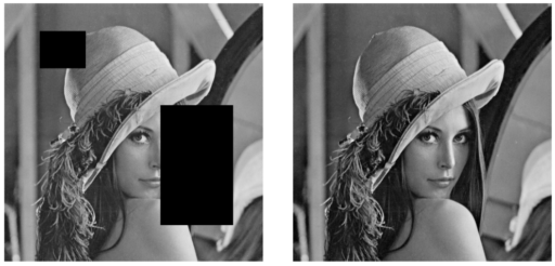
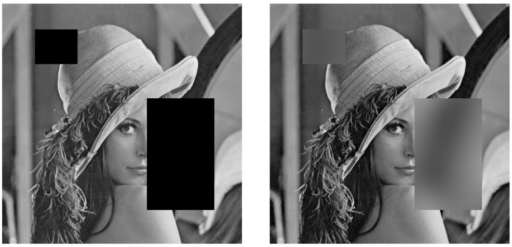
This problem in imaging is called inpainting, which simple the idea of complete a missing portion of an image based on the complete context of the surroundings (see figure 4). Classically, simpler non-adaptive interpolation was done in CT, but today more power full algorithms in Machine Learning, known as Conditional Generative Adversarial Nets (cGAN), had emerged in the last couple of years with incredible results.

Figure 4: Inpainting of a missing portion of Lenna in the image, which can be completed based on the context of the surroundings. Note that a simpler non-adaptive interpolation algorithm can’t do a very good job, but a human or a modern ML algorithm can do it much better based on context and their past knowledge of the world.

The U-Net generator

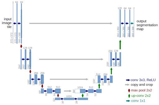
Before modern cGANs, there where some attempts for using directly a U-Net generator for inpainting. Mainly because this kind of U-Net model is very successful in segmentation tasks, in which the output is a binary mask of the same input size, segmenting the objects of interest.[2] So given the success, this U-Net generators make a lot of sense for inpainting tasks, and actually is the main component of a cGAN. U-Net generators have three ingredients that make them successful (see figure 5):

It uses Convolutional layers which had proven to be great for computer vision. Mainly because they reduces a lot the number of parameters in comparison to a fully connected neural network, reducing computation cost and prevents overfiting. It also takes advantage of the translation invariance across an image, and the classical theory of filters by even detecting common things as borders or compressing information which is connected with the frequency domain (the Fourier Transform).
It has skip connections for preserving information to the last layers, this prevents the evanescent gradients problem and makes it possible to construct a Deep Learning architecture, which gives the capability of learning much more complex patterns than a simpler smaller model.
The model is an auto-encoder, composed of an encoder for the input and a decoder for the output. It gets narrower as it gets closer to the middle, forcing to compress the information and get the relevant features. Then, at the output, the model returns the target to the original input size.

Figure 5: U-net architecture example of the original paper for a segmentation task.[2] Each blue box corresponds to a multi-channel feature map. The number of channels is denoted on top of the box. The x-y-size is provided at the lower left edge of the box. White boxes represent copied feature maps. The arrows denote the different operations.

Conditional Generative Adversarial Nets

For inpainting Machine Learning model, the state of the art are cGAN.[3] This models are a composition of two models, the main one is a generator, typically a U-Net like architecture, and a classifier which is only used in the training stage. So cGAN is a U-Net model but trained differently using a more complex loss function which depends on the classifier.

The problem of training a U-Net model directly, using the typical L1 or L2 loss functions, is that ML models tends to smooth the predictions (see figure 6). In part, this is due to generalize correctly by preventing overfit. The resulting inpainting image tends to be blurry without high frequency details.

Figure 6: U-Net alone inpainting completion of the image. The reconstruction is blurry without high frequency details.

The problem is that in reality is not possible to determine what was exactly in the missing portion of the image, for example to know exactly where every individual hair is going to be in the missing portion of the image, so in minimizing the L1 or L2 norm in the loss function for every pixel leads to a blurry result as the optimal solution for the model. The solution is optimal in a mathematical sense, but it does not look realistic for a human perspective. For human eye the reconstruction looks very artificial and blurry.

To make the reconstruction more realistic is why cGAN introduced a discriminator for the training stage. The role of the discriminator is to be like human judge for determine when a reconstruction looks realistic and not blurry, going a little against the L1 or L2 loss. In trying to generate realistic results for the discriminator, U-Net is forced to generate highly detail reconstructions. Both the generator and the discriminator competes against each other.

Given there is not a single simple loss function, in the sense that is composed of two kind of opposite parts. The calibration is very hard and actually it doesn’t exist a single metric for which to look to optimize, so we only have a subjective metric. This makes it very hard to tune hyperparameters and find the exact optimum between under and over fitting.

A way to go, is to calibrate the hyperparameters for the U-Net model alone with a classical regression loss, without the discriminator, and use transfer learning for both models (generator and discriminator), even freezing some layers, to finally start calibrating using a more subjective human eye calibration for the hyperparameter $\lambda$ (which controls the importance in the loss function between both model). This makes much more easy to finally calibrate the cGAN.

Formalizing cGAN mathematics

Given $x$ the input image, $m$ the mask of the part of $x$ to complete in the inpainting task, and $y$ the ground truth final target image. Also, naming the U-Net generator as $G(x,m)$ (see figure 7) and the discriminator as $D(x,\_)$ , where the input $x$ is just pass to the discriminator for better performance. Then, the optimal generator $G^*$ is the result of the optimal solution between both loss functions (4) and the classical L2 regression loss (5), as can be see in equation (6). Noting that $\lambda$ is just an hyperparameter which balance both loss functions, and $\mathbb{E}[\_]$ is just the expected value (the mean value across the samples).

Figure 7: The inpainting generator schema, where only the metal traces $m$ are completed forcing to preserve the original for non metal parts $1-m$ . Mathematically $G(x,m) = m\cdot \text{UNet}(x) + (1-m)\cdot x$ .

(4) $\begin{equation*}\mathcal{L}_{\text{cGAN}}(G,D) = \mathbb{E}_{x,y}[\log D(x,y)] + \mathbb{E}_{x,m}[\log (1-D(x,G(x,m)))] \end{equation*}$

(5) $\begin{equation*} \mathcal{L}_{L2}(G) = \mathbb{E}_{x,y,m}[{||y - G(x,m)||_2}^2] \end{equation*}$

(6) $\begin{equation*} G^* = \arg \min_G \max_D \mathcal{L}_{\text{cGAN}}(G,D) + \lambda \mathcal{L}_{L2}(G) \end{equation*}$

Realistic 3D Modeling

Machine learning relies on data to learn. The math and theory might be best, but if the data quality is not good, the algorithm will not work properly or be unreliable. There is a lot of public CT data available in the web, the ones used in here can be found in [4] and [5].

To make the dataset for training, the procedure was first to generate accurate 3D models of the spine, with 3D slicer for segmentation, and then use 3D Studio Max for introducing realistic metal screws and rods as a surgeon will do (see figure 8).

Figure 8: Realistic metal positioning over a 3D model that was get from a CT image. Then the metal can be put back into the image to finally generate the metal artifacts for training. Leading to having the input $x$ with artifacts and ideal target with the clean image $y$ .

Then, metals can be included in the original image volume now in a realistic position and shape obtained by the 3D modeling. Finally, the Radon Transform with the missing metal traces can be generated (see figure 9). With this we have now the ground truth for the original image and the input with the metal traces.

Figure 9: In the image can be see the contrast between our realistic metal positioning, against the random common approach. Notice that the regions to complete in the Radon Transform are quite different from each other.

Discussions

In practice, the realistic approach can also be combined with the more common random approach used in other works to train a more robust model, helping it to predict correctly in more general situations which could be uncommon.

In this project the model only have access to modify the missing information of the metal traces in the Radon Transform space, this ensures that the model will not generate fake elements in the image. This is because to create a fake element in the image space it requires to alter almost every pixel in the Radon space. But the model does not have access to everything and can only modify the lost information in the metal traces of the Radon space.

Also, there is a great similarity between each of the adjacent slices. This is mainly because the thickness of the screws is be very narrow, but the problem is they are placed in the same plane of the slice and then use much more space in the 2D Radon Transform. So it is much better to use the 3D information between adjacent slices for helping in the reconstruction, given much more context to the cGAN model which has not problem in managing (512, 512, 3) 3D dimension inputs (it is a standard of the industry that every slice of a CT volume is of dimensions 512 x 512).

This method also has the advantage of being a post-acquisition algorithm. Therefore, in principle, it is not necessary to have direct access to the CT machine code or any other physical modifications to the X-ray source or the detector. This is a great advantage over other techniques, for example, dual CT can minimize metal artifacts, but not all clinical centers have this type of machine. For a more personal example, when I worked on Compressed Sensing for Magnetic Resonance Imaging it required altering the way the machine performs the acquisition, which is not easy, it requires direct access to the machine code (which is not always possible, and needs special permissions from an ethical and security perspective).

I have this idea for a project many years ago, actually I advanced very much over the years but it is a lot of work for a single person, and I don’t currently work in this field of research for now at least (even though I simply love it). Given that I don’t have the time to finish the project, and that I have the idea for many years now, I prefer to publish it now before it is too late. I have all the codes, theory and make a lot of successful in simply experiments but only need time and resources to finish everything. But for now I prefer to share the method to help the community.

REFERENCES

[1] M. U. Ghani and W. C. Karl, “Fast accurate CT metal artifact reduction using data domain deep learning,” CoRR, vol. abs/1904.04691, 2019. [Online]. Available: http://arxiv.org/abs/1904.04691

[2] O. Ronneberger, P. Fischer, and T. Brox, “U-net: Convolutional networks for biomedical image segmentation,” CoRR, vol. abs/1505.04597, 2015. [Online]. Available: http://arxiv.org/abs/1505.04597

[3] P. Isola, J. Zhu, T. Zhou, and A. A. Efros, “Image-to-image translation with conditional adversarial networks,” CoRR, vol. abs/1611.07004, 2016. [Online]. Available: http://arxiv.org/abs/1611.07004

[4] H. M. Jianhua Yao, Joseph E. Burns and R. M. Summers, “Detection of vertebral body fractures based on cortical shell unwrapping,” International Conference on Medical Image Computing and Computer Assisted Intervention, vol. 7512, pp. 509–516, 2012.

[5] M. Jun, G. Cheng, W. Yixin, A. Xingle, G. Jiantao, Y. Ziqi, Z. Minqing, L. Xin, D. Xueyuan, C. Shucheng, W. Hao, M. Sen, Y. Xiaoyu, N. Ziwei, L. Chen, T. Lu, Z. Yuntao, Z. Qiongjie, D. Guoqiang, and H. Jian, “COVID-19 CT Lung and Infection Segmentation Dataset,” Apr. 2020. [Online]. Available: https://doi.org/10.5281/zenodo.3757476

Tools: Python, NumPy, TensorFlow, Keras, CUDA/GPU, 3D Slicer, 3D Studio Max, SciPy, Matplotlib, Scikit-Image.